Machine Learning - Versus

Last Updated: 2021-11-19

Type I Error vs Type II Error

Type I Error: False Positive
Type II Error: False Negative

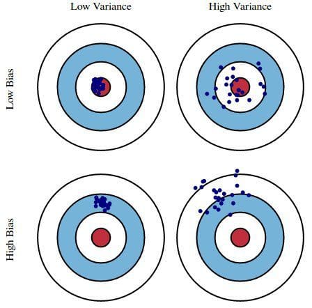
Bias vs Variance

High bias, low variance: models are consistent but inaccurate on average
High variance, low bias: models are accurate on average but inconsistent

Trade-off:

Low variance algorithms:
- less complex, simple underlying structure,
- e.g. Naive bayes, linear algorithms.
- Regularization to further reduce complexity.
- underfit
Low bias algorithms:
- more complex, flexible underlying structure,
- e.g. Decision Trees, Non-linear algorithms.
- Decision Trees can be pruned to reduce complexity.
- overfit

Total Error = Bias^2 + Variance + irreducible error

Image from kdnuggets

Underfit vs Overfit

underfit = high bias
overfit = high variance

regularization parameter : too large, under fit

Accuracy vs Precision

Similar to Bias vs Variance

https://en.wikipedia.org/wiki/Accuracy_and_precision

GBM vs XGBoost

Same:

Both xgboost and gbm follows the principle of gradient boosting.

Different:

xgboost used a more regularized model formalization to control over-fitting, which gives it better performance.

https://xgboost.readthedocs.io/en/latest/

Data Mining vs Database Querying

Database Querying: "What data satisfies this pattern (query)?"
Data Mining: "What patterns satisfy this data?"

Naive Bayes vs Logistic Regression

Naive Bayes ‐ generative model: $P(X|y)$

makes strong conditional independence assumption about the data attributes
When the assumptions are ok, naïve bayes can use small amount of training training data and estimate estimate a reasonable reasonable model

Logistic regression ‐ discriminative model: directly learn $P(y|X)$

has fewer parameters to estimate, learning harder
Makes no strong assumptions
May need large number of training examples

Logistic Regression vs Neural Netowrk

Logistic regression: if use logistic sigmoid functions as activation functions, it is essentially the same as a one layer neural network.

Although neural networks (multi-layer perceptrons to be specific) may use logistic activation functions, the hyperbolic tangent (tanh) often tends to work better in practice, since it’s not limited to only positive outputs in the hidden layer(s).

One of the nice properties of logistic regression is that the logistic cost function (or max-entropy) is convex, and thus we are guaranteed to find the global cost minimum. But, once we stack logistic activation functions in a multi-layer neural network, we’ll lose this convexity.

in practice, backpropagation works quite well for 1 or 2 layer neural networks (and there are deep learning algos such as autoencoders)

ANOVA vs T-test

ANOVA: more than 2 categories in target
z-test, t-test: 2 categories in target

Anova tests use variances to know whether the means are equal or not.

ANOVA and Regression

both continuous outcome variable

Regression model: based on one or more continuous predictor variables.
ANOVA model: based on one or more categorical predictor variables.

NN vs SVM

NN: Empirical Risk Minimization, local minima, overfitting
SVM: Structural Risk Minimization, global and unique

ANOVA vs Discriminant Analysis

ANOVA uses categorical independent variables and a continuous dependent variable
Discriminant Analysis has continuous independent variables and a categorical dependent variable

probit vs logit

http://stats.stackexchange.com/questions/20523/difference-between-logit-and-probit-models

Bagging vs Boosting

Bagging: equal weight for all models
Boosting: the more successful models receive heavier weights

Label Transformation

random forest: no transformation needed for labels
neural net: one-hot transformation

KS vs Chi-squared

Similarities:

Both chi-squared and K-S will give a probability of rejecting the null hypothesis.

Differences:

Chi-squared test: compare binned data (e.g. a histogram) with another set of binned data or the predictions of a model binned in the same way. Artificially binning data loses information, should be avoided if possible.
K-S test: applied to unbinned data (i.e. only one object in each bin) to compare the cumulative frequency of two distributions or compare a cumulative frequency against a model prediction of a cumulative frequency.

Data Parallel vs Model Parallel

From Tensorflow white paper.

Data Parallel

Data Parallel Training One simple technique for speeding up SGD is to parallelize the computation of the gradient for a mini-batch across mini-batch elements. For example, if we are using a mini-batch size of 1000 elements, we can use 10 replicas of the model to each compute the gradient for 100 elements, and then combine the gradients and apply updates to the parameters synchronously, in order to behave exactly as if we were running the sequential SGD algorithm with a batch size of 1000 elements. In this case, the TensorFlow graph simply has many replicas of the portion of the graph that does the bulk of the model computation, and a single client thread drives the entire training loop for this large graph. This is illustrated in the top portion of Figure 7. This approach can also be made asynchronous, where the TensorFlow graph has many replicas of the portion of the graph that does the bulk of the model computation, and each one of these replicas also applies the parameter updates to the model parameters asynchronously. In this configuration, there is one client thread for each of the graph replicas. This is illustrated in the bottom portion of Figure 7.

Model Parallel

Model Parallel Training Model parallel training, where different portions of the model computation are done on different computational devices simultaneously for the same batch of examples, is also easy to express in TensorFlow. Figure 8 shows an example of a recurrent, deep LSTM model used for sequence to sequence learning, parallelized across three different devices. Concurrent Steps for Model Computation Pipelining Another common way to get better utilization for training deep neural networks is to pipeline the computation of the model within the same devices, by running a small number of concurrent steps within the same set of devices. This is shown in Figure 9. It is somewhat similar to asynchronous data parallelism, except that the parallelism occurs within the same device(s), rather than replicating the computation graph on different devices. This allows “filling in the gaps” where computation of a single batch of examples might not be able to fully utilize the full parallelism on all devices at all times during a single step.

Manifold vs Euclidean

In general, any object that is nearly "flat" on small scales is a manifold.

Is the Earth flat or round?

The ancient belief: the Earth was flat
The modern evidence: it is round. On the small scales that we see, the Earth does indeed look flat.

AdaBoost vs Gradient Boosting

AdaBoost: short for Adaptive Boost.

Same: Both are boosting algorithms: convert a set of weak learners into a single strong learner. Both initialize a strong learner and iteratively create a weak learner that is added to the strong learner.

Diff: how they create the weak learners

AdaBoost:

At each iteration, adaptive boosting changes the sample distribution by modifying the weights attached to each of the instances. It increases the weights of the wrongly predicted instances and decreases the ones of the correctly predicted instances. The weak learner thus focuses more on the difficult instances. After being trained, the weak learner is added to the strong one according to his performance (so-called alpha weight). The higher it performs, the more it contributes to the strong learner.

Gradient Boost

gradient boosting doesn’t modify the sample distribution. Instead of training on a newly sample distribution, the weak learner trains on the remaining errors (so-called pseudo-residuals) of the strong learner. It is another way to give more importance to the difficult instances. At each iteration, the pseudo-residuals are computed and a weak learner is fitted to these pseudo-residuals. Then, the contribution of the weak learner (so-called multiplier) to the strong one isn’t computed according to his performance on the newly distribution sample but using a gradient descent optimization process. The computed contribution is the one minimizing the overall error of the strong learner.

https://www.quora.com/What-is-the-difference-between-gradient-boosting-and-adaboost